Part 4 ended with every learned model beating the DSP baseline on accuracy and none of them fitting the cloud container. That result raises an obvious question: what if the model runs where the audio already is — directly on the ESP32-S3, no upload, no container, no network round trip at all? The constraint there isn't megabytes of container dependencies. It's kilobytes of flash, on a chip that also has to keep sampling audio in real time.
The flash budget, measured before a line of model code was written
The device's flash partition is 1.5 MB total, and the deployed firmware — Wi-Fi, the I2S capture path, the DSP filter chain from Part 1, upload logic, flash queueing — already occupies about 1.05 MB of it. That leaves roughly 450 KB for everything a learned model needs: the TensorFlow Lite Micro interpreter, its operator resolver, and the model's own weights. Not a nominal figure — growing it further would mean shrinking the clip-storage partition, which is already suspected of causing a separate bug (dropped clips when the queue fills), so taking flash from there would make a known problem worse rather than solving this one.
8 MB of octal PSRAM is available for the working memory a model needs at inference time (the "tensor arena"), so that's not the bottleneck. Code and weights, which have to live in flash, are.
Same frontend, proven bit-identical
The mel-spectrogram frontend that turns raw audio into what a model actually sees has to run twice: once in Python during training, and once in hand-rolled C on the device at inference time — no ESP-IDF dependencies, a from-scratch radix-2 FFT, because the model has to run inside the same tight flash budget as everything else. Two independent implementations of the same math is exactly the kind of arrangement that drifts silently if nobody checks it.
So it was checked directly: a golden-vector test comparing the training-side Python frontend against the on-device C frontend, on real captured clips. Largest disagreement measured: 8.34 × 10⁻⁴ — floor noise on the single highest mel frequency bin, the exact signature a small implementation predicted before the test ran. That's the difference between "the model works" and "the model works on the specific numbers it was shown during training, and something subtly different once it's on the chip" — and it's the check most quantisation bugs hide behind.
The architecture, and why it's this small
40×150 log-mel frames feed two convolutional blocks (3×3 kernels, 16 then 32 channels, stride 2, ReLU, max-pool), followed by global average pooling and a single-unit head. Small by design — every layer choice was made against the 450 KB budget, not the other way around.
Quantised to int8, the model weights come to 9.5 KB. Adding the TFLite Micro interpreter and operator resolver brings the total delta to roughly 67 KB — well inside the 450 KB budget, with about 410 KB of headroom left over. That headroom mattered less as a safety margin and more as a sign the constraint had been respected rather than fought: the plan's original estimate for the interpreter overhead had been roughly 2.3× pessimistic, because a hand-picked operator resolver covering exactly the five ops this model needs is a fraction of the size of a resolver that supports everything TFLite Micro can do.
chip_cv_results.json.Training data, and the honesty check that caught a real leak
A small seed set from a public siren dataset (ESC-50, resampled to match the device's 16 kHz mono capture) gave the model a starting point before real window recordings existed in useful volume, then fine-tuning ran on the same day-grouped folds used for the cloud bake-off in Part 4.
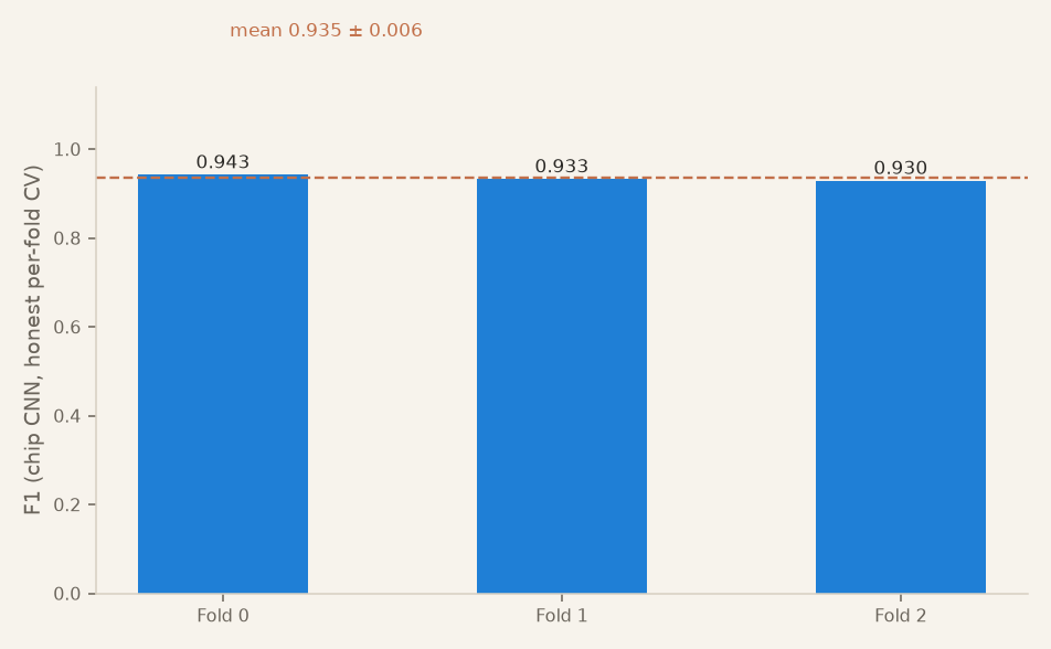
The first evaluation looked excellent — 0.948 mean F1. It was also wrong, in a specific and instructive way: the model being scored had been fine-tuned on two of the three folds it was then evaluated against, so part of that number was the model recognising data it had already trained on. The fix retrains a fresh model per fold, holding one fold out entirely and watching early-stopping against a day held out of the training folds too — never touching the test fold at any point in the process.
The honest result: F1 0.941 ± 0.009, beating the DSP baseline (0.871 ± 0.033) on every individual fold, not just on average. The drop from 0.948 to 0.941 is the cost of closing the leak — small, but the leak was real, and reporting the honest number instead of the leaked one is the only way this comparison means anything.
The transferable bit
A model scored against data it partially trained on will look better than it is, and the gap can be small enough to not look suspicious — 0.948 versus 0.941 doesn't scream "leak" the way a much larger gap would. The only reliable defence is structural: retrain fresh per fold and never let early-stopping see the test fold, rather than trusting that a good-looking number is automatically a real one.
Turning a model in a folder into firmware
A trained, quantised model isn't deployed until it's actually running inference on the chip, end to end, and that step surfaced its own set of traps:
- The TFLite Micro runtime version was pinned exactly — not to the newest release, deliberately. A one-month field trial that has to reproduce months later shouldn't sit on a dependency that was one day old when it was chosen.
- A build with the model present but never called from anywhere is byte-identical to a build without it at all. The linker discards unreferenced code, so simply adding the model files to the project would have silently reported "the model costs zero bytes" right up until the moment something actually invoked it.
- Rounding conventions don't match by default. NumPy's
roundrounds half-to-even; C'sroundfrounds half-away-from-zero. Left unreconciled, this shows up as a small, structured ±1 discrepancy that looks exactly like measurement noise rather than a systematic bug — until someone goes looking for a pattern in what should be random error.
Final firmware size: 1.09 MB against the 1.5 MB partition, with a build-time assertion added so that exceeding the flash budget fails the build immediately rather than failing silently at flash time. A second golden-vector check — this time comparing the device's actual quantised input path against what the training pipeline would have produced for the same audio — passed with a largest disagreement of a single count, well inside tolerance.
The result that mattered: does the chip clear the bar the DSP couldn't?
Operating thresholds for both the DSP and the chip model were frozen out-of-fold — chosen without ever looking at the labels each detector would later be scored against, the same discipline that Part 2's reversal showed was missing the first time around:
| Detector | Threshold | Precision | Recall | Clears 90/90? |
|---|---|---|---|---|
| chip | 0.65 | 93.9% | 94.9% | yes |
| dsp | 0.40 | 84.7% | 86.5% | no |
This isn't the final trial verdict yet — that requires the inverse-probability-weighted estimate from labels collected during a live soak, which is what Part 6 covers. But it's the first time in this whole series that a learned model has actually cleared the bar the DSP set out to meet, on a real, honestly-measured comparison, running on the exact hardware it will ship on.
What made this different from the cloud attempt
The cloud bake-off in Part 4 optimised for accuracy first and discovered the deployment constraint afterward — which is why every candidate there lost on a gate that had nothing to do with modelling skill. This model was built the other way around: the architecture, the quantisation, the flash budget were all decided relative to the constraint from the start, not measured against it as an afterthought. Building to the constraint, rather than fitting a winning model into it after the fact, is the difference between a model that scores well on paper and one that actually ships.
What's next
Two detectors — DSP and chip — now both have honest, out-of-fold numbers, and the chip clears a bar the DSP doesn't. But every number so far comes from pre-soak labels, frozen thresholds tested against data collected before the trial began. The real test is running all of it live, for real, for a month, without touching anything — and reporting whatever actually happens, including if the answer turns out to be "we can't tell." That's Part 6.