By the point the DSP-vs-DSP reversal in Part 2 had happened, it was clear no single number computed in-sample could be trusted. What was needed instead was a labelling design robust enough to compare three different detectors — the hand-tuned DSP, a cloud model, and an on-chip model — fairly, on data none of them had seen. That design turned out to be most of the actual engineering work in this project, and almost none of it is about the model.
Why recall is the expensive metric, not precision
Precision is cheap to measure: sample the clips a detector actually flagged, and check whether they're really sirens. You're looking where the detector is already pointing.
Recall is the opposite problem. To measure it honestly you have to find the sirens a detector missed — and by definition, those live in the part of the corpus every detector scored near zero. In this project's corpus, roughly 83% of clips fall below every detector's own operating threshold. That 83% is where a false negative hides, and it's also the most tedious part of the corpus to label, because almost everything in it really is nothing.
A labelling budget that samples uniformly at random spends most of its 10 minutes a day confirming silence. That's not free — it actively starves the one measurement that determines whether any detector is safe to trust.
Two streams, and why they can never be pooled
The labelling design splits into two independent streams, each answering a different question and neither substitutable for the other.
Stream A — disagreement, ~6 clips/day. Clips where the detectors under comparison score differently. These carry information about which detector is better relative to another, and nothing about how good any one of them is in absolute terms. A clip only ends up in Stream A because it triggered a disagreement — which means it was selected in a way that depends on the detectors' own scores, not independently of them.
Stream B — stratified random, ~14 clips/day. This is where the actual precision/recall numbers come from, and it has to be unbiased. The naive version — sample uniformly — wastes most of its budget on the 83% that's trivially silent. Instead, clips are bucketed into strata by how close their score sits to each detector's own frozen operating threshold, and each stratum gets a fixed daily quota with a known selection probability:
| Stratum (score relative to threshold) | Clips/day | Sampled/day | P(selected) | Why |
|---|---|---|---|---|
| ≥ 1.0 — above some detector's threshold | ~15 | 4 | 27% | Where precision is measured |
| 0.3 – 1.0 | ~16 | 3 | 19% | The ambiguous band |
| < 0.3 — below every detector, with margin | ~150 | 7 | 5% | Where missed sirens hide — this stratum determines recall |
That allocation looks backwards at first glance — the smallest slice of the corpus (the top stratum) gets sampled at 27%, while the largest slice (the bottom, quiet stratum) gets sampled at just 5%. It's deliberate: precision is cheap to measure because the detector already told you where to look, so a small sample there goes a long way. Recall is expensive precisely because you're searching blind through a mostly-empty haystack, so it needs a larger absolute allocation even at a much lower sampling rate. Every sampled clip records its stratum and selection probability, and precision/recall are computed over the whole corpus by weighting each label by the inverse of how likely it was to be picked — inverse-probability weighting, so the 5%-sampled bottom stratum isn't quietly under-represented in the final number.
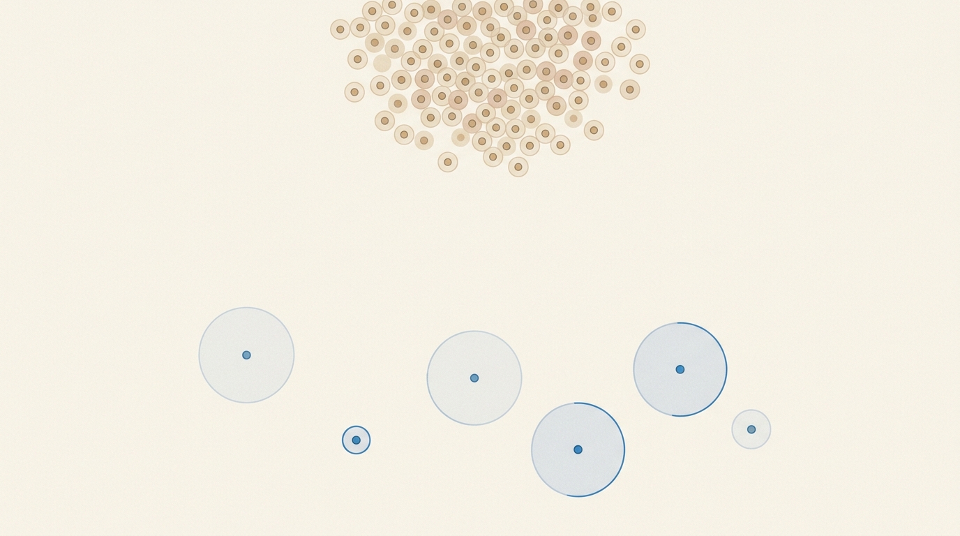
The rule that's easy to get wrong in a hurry
A clip labelled because a detector flagged it (Stream A) cannot be used to estimate that detector's precision without correcting for the fact that it was selected because it scored high. Pooling Stream A and Stream B numbers together silently biases every result toward whichever detector's disagreements got labelled most. They stay separate, always.
Sizing the quota wasn't a guess — it was a simulation
The 7-clips-a-day figure for the bottom stratum came from asking a sharper question than "how many labels feel like enough": how often would a genuinely bad detector — one that actually misses 25% of real sirens — get falsely reported as clearing a 90% recall bar, purely from under-sampling that stratum?
| Low-stratum quota/day | Labels/month | False-CLEAR rate for a 75%-recall detector |
|---|---|---|
| 3/day | 90 | 13.7% |
| 5/day | 150 | 3.0% |
| 7/day (as specified) | 210 | 0.7% |
| 10/day | 300 | 0.7% |
| 15/day | 450 | 0.2% |
The failure mode at low sample counts is specific: the most likely single outcome is observing zero low-band sirens purely by chance, which reports a deceptively perfect 100% recall with a falsely tight confidence interval — not real confidence, just a lucky draw for a genuinely bad detector. Seven a day is roughly where that risk collapses to noise; below it, the risk reopens fast. If daily labelling capacity ever needed to shrink, the slack lives in the top two strata — they serve precision and the arm-to-arm comparison, not the safety-critical recall bound, so they can absorb a cut that the bottom stratum can't.
The honest limit, stated up front
Even with careful sampling, roughly 130 labelled positives were expected over a full month of collection — and the ones that matter most, the bottom-stratum finds that anchor the recall estimate, number somewhere between 4 and 12. That range isn't a guess; it comes from two different estimates that bracket the true value from opposite directions, and the gap between them is the honest uncertainty. A comparison resting on single-digit counts has a genuinely wide confidence interval, and no amount of careful stratification changes that arithmetic — it can only make sure the few labels that exist are spent where they matter.
The exit rule that later decisions get judged against, described fully in Part 6, was written to respect this limit rather than paper over it: a detector only "clears the bar" if both the point estimate and the lower bound of its confidence interval are above the threshold. A detector reading 91% recall with a lower bound of 78% has not cleared the bar — it has failed to be measured precisely enough, and that's reported as a distinct, third outcome rather than quietly rounded up to a pass.
What this buys the rest of the series
None of the model comparisons in Parts 4, 5 and 6 mean anything without this. A bake-off between a cloud model and a hand-tuned DSP detector is only informative if the labels it's scored against weren't implicitly biased toward whichever detector happened to generate them. That's the quiet, unglamorous discipline underneath every accuracy number that follows — and it's also, honestly, the part of this project that took the most design effort relative to how little anyone will notice it in the results table.
With a labelling design that can support a fair comparison, the next question is what to actually compare against the DSP baseline. Part 4 is the first attempt: picking a cloud-hosted model without letting a favourite pick itself.